进阶NLP模型整理(Seq2Seq+Attention+pre_transformer+pre_BERT)

1. 句向量

2. Seq2Seq

采用Encoder和Decoder

Encoder相当于一种压缩器，将最有用的特征识别出来，用最简练的信息表达。
Decoder是解压器，将向量化表达转变为其他表现形式。

2.1 LSTM模型【SimpleRNN】（以机器翻译为例）

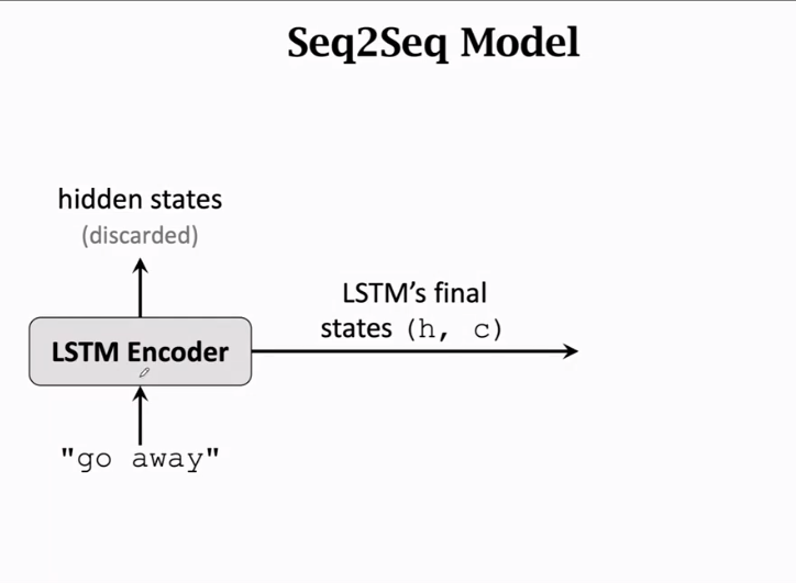
Encoder
- 用于提取特征，最后一个输出即为特征，其他隐藏层被丢弃，输出为最后一个状态h和c
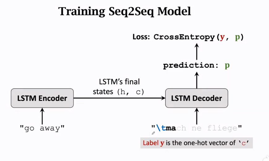
Decoder
- 初始状态为Encoder的最后一个状态
- 每次接受一个输入，然后输出下一个字母的概率，第一个输入为起始符
- decoder输出一个概率分布，结合标签形成一个CrossEntropy函数，梯度从Decoder传回Encoder。
训练及预测过程
- training中，不管有没有预测错，下一步在decoder的输入都是正确的
- inference中，decoder下一步的预测基于decoder上一步预测，而不是true label
提升：
- encoder用双向LSTM，decoder是单向LSTM
- multi-Task learning：多加入几个任务，比如让英语翻译成英语等，这样encoder可以被训练的更好

2.2 Attention(注意力)机制【SimpleRNN+Attention】

2015年提出，用来改进Seq2Seq模型，用来解决遗忘问题
decoder每次更新状态之前，encoder会对整体信息进行softmax(打权重)，从而使decoder了解应加强注意哪些encoder的step上，在结合decoder的输入信息一起训练，这就是Attention名字的由来，同时不会忘记原始输入，但缺点是计算量很大。
原理过程：
1. encoder结束后，attention和decoder同时工作
2. decoder的初始状态\(s_0\)是encoder的最后一个状态，同时encoder的所有状态都要保留
3. 先计算decoder的初始状态\(s_0\)与encoder中每个状态\(h_i\)的相关性，使用\(a_i=aligh(h_i, s_0)\)来计算相关性，结果即为\(a_i\)，记做\(Weight\)（此\(a_i\)是经softmax处理过的）。
4. 计算与\(s_0\)对应的\(a_i\)（计算出的m个\(a\)最后还需经softmax处理得到\(a_i\)）：
  - 第一篇attention论文提出的计算方法
    - \(aligh(h_i, s_0)=v_a^\mathrm{T}tanh(W_a[h_i;s_0])\qquad concat\)
    - \(v_a\)与\(W_a\)都是参数，需要从训练集中学习
  - 更常用的一种方法
    - Linear maps:
      - \(k_i=W_k×h_i\qquad for\ i=1\ to\ m\)
      - \(q_0=W_Q×s_0\)
    - Inner product:
      - \(\tilde a_i=k_i^\mathrm Tq_0\qquad for\ i=1\ to\ m\)
    - Normalization:
      - \([a_i,...,a_m]=Softmax([\tilde a_1,...,\tilde a_m])\)
5. 计算与\(s_0\)对应的Context vector \(c_0\)，加权平均
  
  \(c_0=a_1h_1+...+a_mh_m\)
6. 更新下一个状态\(s_1\)，\(x_1'\)为输入的数据
  - SimpleRNN中 \[ s_1=tanh(A' \begin{bmatrix} x'_1\\ s_0 \end{bmatrix} +b) \] 仅仅根据上一状态，并不会看encoder状态
  - SimpleRNN+Attention中 \[ s_1=tanh(A' \begin{bmatrix} x'_1\\ s_0\\ c_0 \end{bmatrix} +b) \] \(c_0\)是encoder中所有状态\(h_i\)的加权平均，所以\(c_0\)记录有\(x_1\)到\(x_m\)的完整信息，而decoder的更新一来于\(c\)，故RNN的遗忘问题可解决。
7. 再计算\(s_1\)跟之前encoder所有状态的相关性，即\(a\)，再计算\(c_1\)，decoder接受新的输入\(x_2'\)，循环计算下去直至结束。
计算量：为计算\(weight\ a_i\)，共需计算encoder和decoder数量的乘积次，故attention为了不遗忘，是以高数量级计算为代价。
权重\(a\)的实际意义：

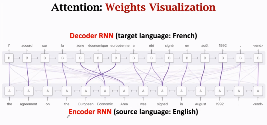
线越粗，相关性越高

2.3 总结

Stardard Seq2Seq model: the decoder looks at only its current state
Attention: decoder additionally looks at all the states of the encoder
Attention: decoder knows where to focus
Downside: higher time complexity
- m: source sequence length
- t: target sequence length
- Standard Seq2Seq: \(O(m+t)\) time complexity
- Seq2Seq+attention: \(O(mt)\) time complexity

3. Transformer

是一个Seq2Seq模型，有一个encoder和一个decoder
完全不是RNN，而是基于attention层、self-attention层、全连接层
输入输出shape与RNN相同

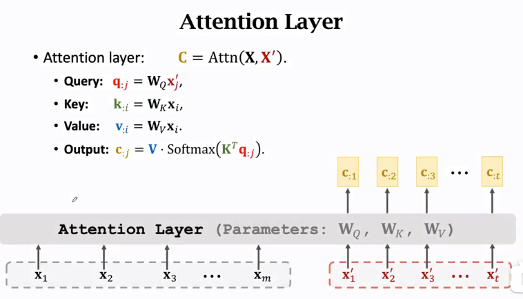
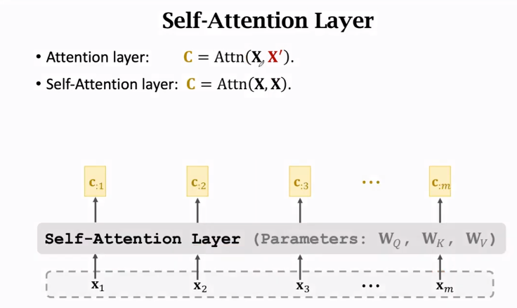
3.1 Attention Layer

Encoder's inputs：\(X=[x_1,x_2,...x_m]\)，每一个输入为d维

Decoder's inputs：\(X'=[x_1',x_2',...,x_t']\)，每一个输入为d维

Parameaters：\(W_Q, W_K,W_V\)

\(C=Attn(X,X')\)

Query：\(Q=W_QX'\)	Key：\(K=W_KX\)	Value：\(V=W_VX\)
\(W_Q:q×d\) \(X':d×t\) \(Q:q×t\) 【Q中每一列对应一个\(x'\)】	\(W_K:k×d\) \(X:d×m\) \(K:k×m\) 【K中每一列对应一个\(x\)】	\(W_V:v×d\) \(X:d×m\) \(V:v×m\) 【V中每一列对应一个\(x\)】

Weights：\(a=Softmax(K^TQ)\) 【k=q，\(a:m×t\)】

Context vector：\(C=Va\) 【\(c:v×t\)，每一列对应一个\(x'\)】

\(K\)与\(V\)是对应于encoder，\(Q\)是对应于decoder层，最后输出为\(c\)
Output of attention layer: \(C=[c_{:1},c_{:2},...,c_{:t}]\)

Here, \(c_{:j}=V·Softmax(K^Tq_{:j})\)

Thus, \(c_{:j}\) is a function of \(x'_j\) and \([x_1,...,x_m]\)
对比SimpleRNN+Attention的Seq2Seq：
- SimpleRNN：对于decoder层的每一个时间步，需先计算此状态与encoder各层的\(a\)，再计算context vector \(c\)，然后结合上一状态、\(c\)、这一层的输入\(x\)，生成下一状态，继续计算，是一步一步的。
- Transformer：直接将decoder层的输入进行处理生成Q，然后encoder层处理生成K、V，即可直接进行运算得到context vector \(c\)，而无需再一步一步计算。

3.2 Self-Attention Layer

不仅局限于Seq2Seq，可用在所有RNN上，如果只用在一个网络则叫做Self-Attention，2016年提出。
之后发现根本不需要RNN，直接用Attention反而效果更好，由此提出了Transformer模型
Self-Attention Layer：\(C=Attn(X, X)\)

inputs：\(X=[x_1,x_2,...x_m]\)

Parameters：\(W_Q,W_K,W_V\)

3.3 Multi-Head (Self-)Attention

Single-Head：单头，前文讲的
Multi-Head (Self-)Attention
- Using \(l\) single-head (self-)attentions (which do not share parameters.)
  - A single-head self-attention has 3 parameter matrices：\(W_Q,W_K,W_V\)
- Concatenating outputs of single-head self-attentions
  - Suppose single-head self-attentions' outputs are \(d×m\) matrices
  - Multi-head's output shape: \((ld)×m\)

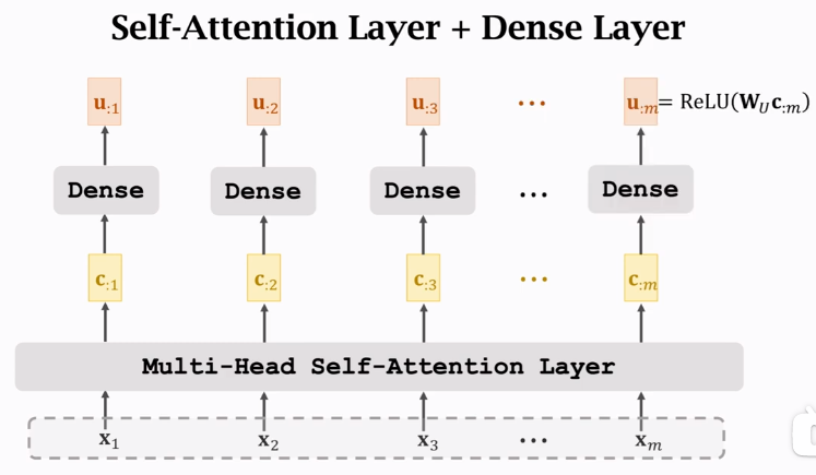
3.4 Stacked Self-Attention Layers【Encoder】

构建Encoder层
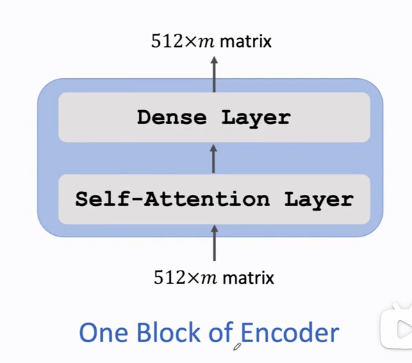
- One Block of Encoder
  
  由两层组成，每个Dense共享一个\(W_U\)，激活函数为\(ReLU\)。输入与输出shape相同。每个\(u\)依赖于所有\(x\)。
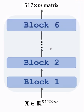
- Stack Blocks
  
  组成Encoder，共6个Block，每个Block两层，每个Block有自己的参数，Blocks之间不共享参数，输入与输出shape相同

3.5 Stacked Attention Layers【Decoder】

构建Decoder层
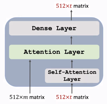
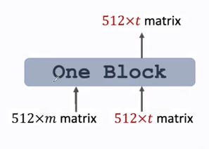
- One Block
  
  由三层组成，有两个输入序列，Dense激活函数也为\(ReLU\)
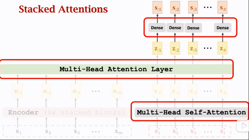
- Transformer's Decoder: One Block【注意图中输入输出shape特点】

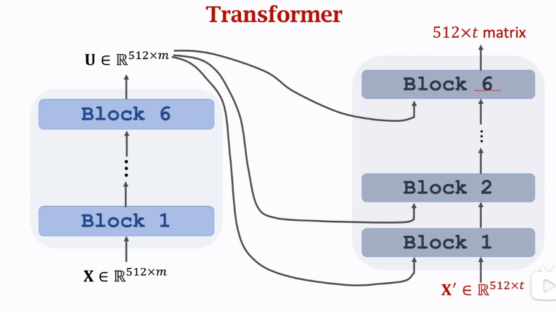
3.6 Put together【Transformer】

左边为Encoder，右边为Decoder，组合起来就是Transformer模型。最终输出为\(512×t\ matrix\)
Comparison with RNN Seq2Seq Model

4. BERT(Bidirectional Encoder Representations from Transformers)

18年提出，19年发表[Devlin, Chang, Lee, and Toutanova. BERT: Pre-training of deep bidirectional transformers for language understanding. In ACL, 2019.]
目的：预训练Transformer模型的encoder网络
- 预训练模型：大规模深度学习模型特点是大、参数多，但是效果提升会更显著，同时不会很容易随着一点变化而完全跑偏，比小模型更容易做迁移。但是训练大模型需要花费的时间很长，所以一个预训练模型很重要，基于预训练模型，我们手头只有小数据集也能得到一个好模型，同时训练速度大大提高，不是从零开始。
- 预训练模型：ELMo、GPT、BERT
两个任务：Predict masked word. Predict next sentence

4.1 Randomly mask a word

随机遮挡词替换为Mask，输出\(u_M\)经Softmax即可得到概率值，可通过概率值判断遮挡的词是什么。
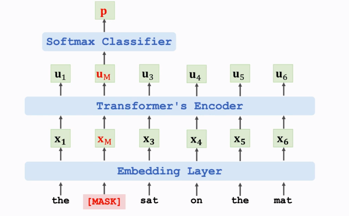
\(e\): one-hot vector of the masked word "cat"

\(p\): output probability distribution at the masked position

\(Loss = CrossEntropy(e, p)\)

Performing one gradient descent to update the model parameters.
为防止机器将mask当成一个词去训练，具体替换方式为：随机选取15%的词做如下改变
- 80%的时间，将它替换成[MASK]
- 10%的时间，将它替换成其他任意词（错别字）
- 10%的时间，不变
预训练不需要人工标注的数据集，可自动生成标签，即可使用维基百科等数据去训练模型，可训练出非常大的模型

4.2 Predict the Next Sentence

分类：[CLS] is a token for classification.

分隔符：[SEP] is for separating sentences.
向量\(c\)在\([CLS]\)的位置上，但并不只依赖于\(c\)，向量\(c\)包含两部分的全部信息。

可以采用\(CrossEntropy\)来构建损失函数
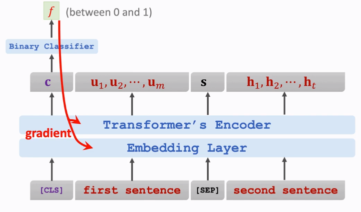
用处：使Embedding词向量包含上下两句话之间的关联信息。Encoder网络中的self-attention层就是寻找相关性，也可使self-attention层找到正确的相关性。

4.3 Combining the two methods

两个任务，对应不同的loss function

Objective function is the sum of these loss functions

Update model parameters by performing one gradient descent